We are now going to start looking at algorithms. An algorithm is, as we have seen, a clearly-defined solution to a particular problem, which follows a series of clearly-specified steps. Common examples of algorithms include sorting collections of data, or searching for an item in a collection of data.

We will start by looking at algorithm efficiency using the Big O notation, and then look at some sorting and searching algorithms, comparing their efficiency.

Algorithm efficiency: the "Big O" notation

When designing algorithms, we need some measure of how complex an algorithm is. Complexity can be measured in various ways, for example performance (time taken), or memory usage. The standard for measuring algorithm complexity is known as the Big O notation. This is a measure which expresses complexity in relation to some property n. This property depends on exactly what we are trying to do. For a sorting algorithm, which sorts a list, for example, it could be the number of items in the list. For indexing a list or linked list, it could also be the number of items in the list; the larger the list, the more items we potentially have to traverse to reach a given index.

"Big O" notation is expressed in terms of this property n. For example we can have:

• O(1) : if an algorithm is O(1) it means that its complexity is independent of n.

• O(n) : if an algorithm is O(n) it means that its complexity depends on the value of n directly, or linearly. So if n increases by 2, the complexity will also increase by 2.

• O(n^2) (^ indicates "power"): if an algorithm is O(n^2) then the time taken or memory used is most influenced by the square of the number of items. So if the number of items doubles, then the time taken will increase around four times. Or if the number of items increases by 10, the time taken will increase around 100 times.

Algorithms which have an outer and inner loop, in which we have to loop through an array twice, are of this kind. The outer loop has to be run n times, but the inner loop has to be run n times each time the outer loop runs. So the time taken is proportional to n^2. For example, below is some code with two loops, an outer and inner loop. An algorithm do_something() is performed n^2 times (16 times in the example, as n is 4). If n is changed to 5, then the operation will be performed 25 (5^2) times.

Answer to exercise 1

Calculating the memory address of the index of an array would be an example of an O(1) operation because it is always given by the equation:

Clearly the time taken to evaluate this equation does not depend on the size of the list, which is the property n in this case. Even if the list is very large, and the index is very large, we can quickly calculate the item's address using the simple equation above. O(1) algorithms are thus highly efficient… but not many algorithms are O(1)!

Likewise, adding a new item to a linked list would also be O(1) as the time taken does not depend on the length of the linked list. This is because we always have a reference to the last node, and we can link the item to the last node immediately.

Looking up an item in a hash table with no collisions (clashes) would also be O(1). We simply convert the key to a hash code using a hash function, and then obtain the bucket by taking the modulo of the number of buckets of the hash code. None of this is dependent on the number of items in the hash table.

Indexing a linked list is a good example of an O(n) algorithm because we have to manually follow the links to retrieve the item with a given index - we cannot rely on consecutive memory addresses. So complexity of linked list indexing is related linearly to the length of the list.

A basic search for an item in a list, in which we loop through all members of the list until we find the search term we are looking for, is also O(n): it's again linearly related to the length of the list, because in a worst-case scenario, we will have to search through the entire list before we find the item. This type of search is known as linear search.

This brings up an important point, the big O notation used is the worst-case scenario. In a basic search such as this, we assume the index will not be found until the end of the list in which case we will have to search through n items, where n is the number of items in the list.

Performing a transformation on each pixel in a square image would be O(n^2) with respect to the dimension of the image, n. We'd need an outer loop to loop through each row of pixels, and an inner loop to loop through each pixel within the current row. So as n increases, the number of operations increase proportional to the square of n.

More on O(n^2) algorithms

Clearly it can be seen that O(n^2) algorithms are not efficient, and should be refactored to a more efficient algorithm e.g. O(n) or, as described below, O(log n).

O(n^2) algorithms are known as quadratic because their complexity can be calculated using a quadratic equation an^2 + bn + c. It should be noted that, depending on the exact algorithm, the complexity will not be exactly n^2. However it will be something close to n^2 which can be expressed using a quadratic equation. If you consider a quadratic equation, it can be seen that, as the variable n increases, the n^2 term will come to predominate the result.

for the value n=100 will be:

which is

It can be seen that the n^2 term predominates. Remember we said above that in Big O notation, we need to worry about worst-case scenarios (scenarios with large n typically) as these will be the main source of inefficiencies. So it can be seen that, in these worst-case scenarios, even if the complexity is not exactly n^2, it will approximate to it. So, such algorithms are still designated O(n^2).

Essentially, when considering complexity with the Big O notation, we divide algorithms into classes, and ask ourselves which class (e.g. O(1), O(n), O(n^2) etc) does the algorithm fall into, depending on the behaviour of the algorithm for large n. We are less interested in an absolute value for the time taken, or memory used, to complete an algorithm and more interested in the algorithm's behaviour for very large values of n, so we can see what happens in worst-case scenarios.

The diagram below shows how complexity increases with increasing n for different classes of Big O complexity.

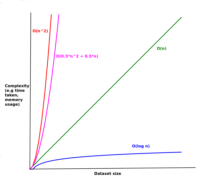
• n is along the x (horizontal) axis, while the complexity is along the y (vertical) axis;
• green is O(n);
• red is O(n^2);
• blue is O(log n); to be discussed below;
• magenta is the quadratic equation 0.5*n^2 + 0.5n. This shows that the quadratic form is exhibited, and the shape of the graph, with a rapid increase with the rate of increase getting bigger with larger values of n is very similar to n^2. (This is known as a parabolic graph). So, even if the complexity is not exactly O(n^2), the behaviour of the graph for increasing n is essentially the same as O(n^2).

Logarithmic complexity

If an algorithm is O(log n) it is related to the logarithm of n. Logarithm is the inverse operation to power, and is always expressed in terms of a particular base. A logarithm of a given number (relative to a particular base, such as base 10 or base 2) will give you the power the base has to be raised to, to give that number. So if b to the power p equals x, then log(b)x = p.

In Big O notation, the base is 2. So for example, if:

so:

Hopefully you can see from this that an O(log n) operation is relatively efficient, because we can increase n significantly but the time taken, or memory consumed, will increase much less. For example, to perform an O(log n) operation on a list of 256 (2^8) items will only take twice as long as a list of 16 (2^4) items. Constrast that to an O(n) algorithm which will take 16 times as long (because 16 x 16 is 256). So if you can refactor an algorithm from O(n) to O(log n), it is clearly desirable.

You should be able to see that an O(log n) operation has an initial fast increase in complexity which then flattens out. Algorithms which involve one complex operation which must be done once, or a small number of times, no matter what the value of n, followed by a less-complex operation, will typically be of the form O(log n).

Introduction to sorting algorithms

We are now going to start looking at sorting algorithms, and consider the Big O complexity of each algorithm we examine.

Bubble sort

We are now going to look at various sorting algorithms and express their complexity in Big O notation. The first algorithm we will look at is the bubble sort. This is a simple algorithm, but it is not very efficient and generally not recommended. Nonetheless, we will start with it as it is simple and provides a simple case to discuss algorithm complexity. As you can see from the diagram below, it involves looping through a list and considering each pair of values in turn. If the pair is in the correct order, we do nothing. If it is not, we swap them.

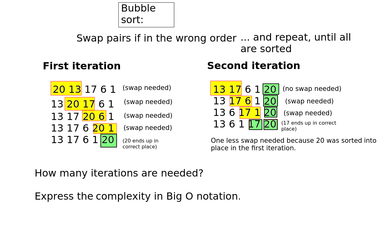
As you can see from the diagram, larger numbers move towards the end of the list, for example the value 20 will, each time a swap is done, move one position onwards in the list. So once we've finished the first iteration of the sort, the largest value will be in the correct position.

So we then need to iterate (loop) again through the list, and perform another series of swapping operations. You can see this on the "second iteration" part of the diagram.

We'd therefore need to implement this using a loop within a loop. The outer loop would be the successive iterations, whereas the inner loop would be used to perform the swapping operations of one particular iteration of the algorithm.

It should be noted that at the end of the first iteration of the bubble sort, the largest value will be correctly in place at the end of the list. So on the second iteration, we do not need to consider the last position in the index; for example if there are 5 values, we only need to consider the 4 smaller values in the second iteration. Similarly, at the end of the second iteration, the second-biggst value will be correctly placed, so on the third iteration we do not need to consider the final two values of the list.

Swapping variables

As we have seen, we need to swap adjacent values if they are in the wrong order. We cannot just do:

because the first statement will set a to b and overwrite the original value of a, so both a and b contain the original value of b. So, when we execute the statement b = a we will uselessly set b to its original value, because a now contains the original value of b.

We could use a temporary variable to store a before assigning the variable a to the value of b, which means we do not lose the original value of a.

However, in Python there is a shortcut for swapping variables which does this for us without needing to declare a temporary variable:

Answer to exercise 2

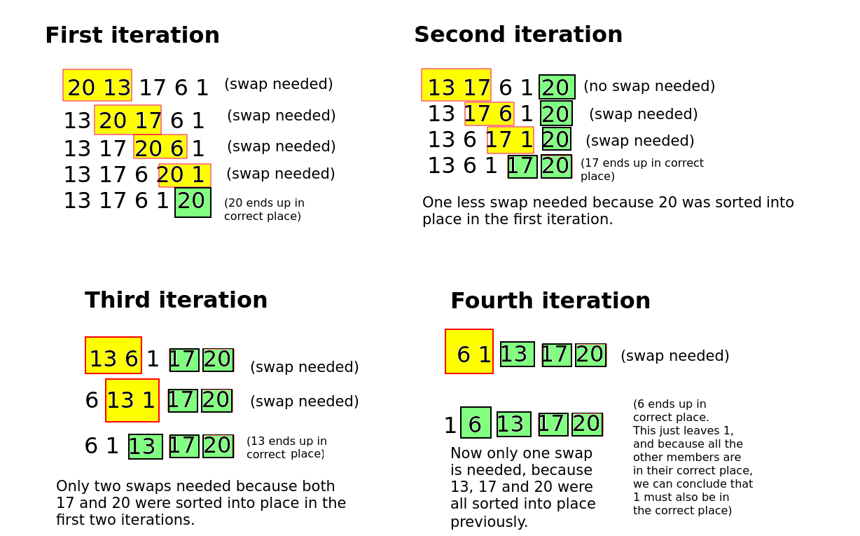
The diagram above shows the full bubble sort algorithm.

Answer to exercise 3

Number of iterations needed for bubble sort

It can be seen that a total of four iterations are needed, in other words the size of the data (5) minus one. This will always be true with bubble sort: the number of iterations needed will be n-1 where n is the dataset size.

Why is this? You should be able to see from the diagram above that each iteration of bubble sort sorts one item into its correct place. So if we move through the list one pair of numbers at a time, the largest value will always move to the end of the list.

So the first iteration sorts the largest item into place, and the second iteration sorts the second largest item into place and so on.

Eventually we will reach iteration n-1 (e.g. iteration 4 for a dataset size of 5) and the n-1 largest items will be sorted into their correct place (e.g. the largest 4 if there are 5 items). However if the n-1 largest items are sorted into their correct place, the remaining item, i.e. the smallest item, must be before them, i.e. at the start of the list. Therefore it too must be in its correct place, and therefore the entire list is sorted. So we only need n-1 (not n) iterations.

How many swaps are needed per iteration?

With bubble sort we have n-1 iterations, but within each iteration we perform a series of swaps. So we need a loop within a loop - an outer loop for the iterations, and an inner loop for the swaps. But how many swaps are needed for a given iteration?

For the first iteration, n-1 swaps are needed. Because we swap two values, the number of swaps will be the dataset size (n) minus one. The first pair will be members 1 and 2, the second pair members 2 and 3, and the final pair therefore will be members n-1 and n. (We are numbering members from one, not zero). So we need n-1 swaps.

On the second iteration, we need one less swap as the diagram shows, because the largest item is already sorted into its correct place. So we'll only need n-2 swaps, i.e. one less than n-1.

On the third iteration we need n-3 and so on.

So if we generalise this, we need n-i swaps for iteration i (again assuming we are counting from one, not zero).

What is the complexity?

As n increases, you need both more iterations and more swaps per iteration. The total number of swaps needed is the number of iterations multiplied by the number of swaps per iteration, so it can be seen that the total number of swaps increases by a greater factor than the increase in dataset size. So the complexity must be worse than O(n), because if it was O(n) the number of swaps would increase proportionally to the dataset size.

We can see from the discussion above that the total number of swaps needed is given by

So the total number of swaps is in fact the sum of all integers from n-1 to 1, descending. So for a dataset of 5, the number of swaps is 4+3+2+1 = 10. For a dataset of 6, the number of swaps is 5+4+3+2+1 = 15.

What complexity is this though?

Mathematically, the sum of all integers from 1 to any integer x is always given by the equation:

You should recognise this from the discussion above as a quadratic equation. Therefore, bubble sort must be O(n^2).

However, as we have seen, it is often not necessary to calculate the exact complexity for any given algorithm. Instead, in many cases you should be able to give the algorithm a complexity class (or order) by looking at how it works.

Any algorithm involving a loop within a loop, where both loops depend on the dataset size and the inner loop performs a computationally-expensive operation, will be O(n^2), even if the loops don't need to iterate through all the values. The increase in the number of operations as the dataset size increases will be mostly governed by the n^2 term, as we saw above.

Any algorithm involving a single loop performing the computationally-expensive operation, where the loop depends on the dataset size, will be O(n).

Coding Exercise 1

Have a go at coding bubble sort in Python. You should create a list of numbers to sort, and once the algorithm has finished, print the list to test whether the sort has taken place. If you are struggling, try writing it in pseudocode first.

Selection sort

Selection sort is another sorting algorithm which is conceptually simple but (relatively) inefficient. Nonetheless it has some advantages over bubble sort, in particular, the number of swap operations is minimised (of order O(n) rather than O(n^2)), and will be used as another example of a sorting algorithm.

How does selection sort work?

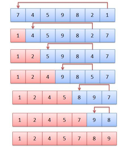
We once again have an outer loop. This loops through each member of the list (apart from the last). Within the outer loop we have an inner loop which compares the current member with each of the remaining members in turn. The lowest remaining member is found, and if this is lower than the current member, the current member and this lowest member is swapped.

See the diagram below, which is based from notes provided by my former colleague Brian Dupée, which were in turn sourced from the former site sorting-algorithms.com (which appears to no longer exist in this form).

It is of interest what this algorithm's time complexity equals, as it raises an important conceptual point about the Big O notation. If you imagine sorting 5 values, what needs to be done?

• The outer loop needs to perform n-1, or 4 swaps.
• The number of operations the inner loop needs to do, depends on where we are in the outer loop. So for the first iteration of the outer loop, we will need to loop through members 1-4 (starting at 0 for the first member) and compare them with member 0. For the second iteration, we need to loop through members 2-4 and compare them with member 1. For the third iteration, we loop through members 3 and 4 and compare them with member 2, and for the fourth iteration, we compare member 4 with member 3.

So the total number of operations for a 5-member list is 4+3+2+1, or more generally for an n-member list, the number of operations is the sum of all the numbers from 1 to n. This value is equal to (n + n^2) / 2.

As we saw for bubble sort, this is an equation of quadratic form, as it can be expressed instead as 0.5n^2 + 0.5n. So with large n values the n^2 term will predominate, and thus, this is an O(n^2) class of algorithm, i.e. less efficient. It is not quite as inefficient as bubble sort, particularly given that less swaps are involved (swapping is a relatively expensive operation as it requires a temporary variable to be created), but it can still potentially be improved.

When swapping numbers, swapping is not particularly computationally expensive. However, if the two values are complex objects which take time to initialise, then the fact that we need to create a temporary variable can mean a swap is expensive. So in cases like this, selection sort is particularly favoured over bubble sort.

Coding Exercise 2

Have a go at implementing selection sort in Python.

Insertion sort

A third type of simple sort, with complexity O(n^2) in many cases, but occasionally O(n) (see below), is the insertion sort. This is shown on the diagram below.

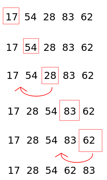
Insertion sort works by progressively inserting values into the list at the correct place. A typical implementation will work through a list and sort it in-place (i.e. within the original list, rather than creating a new list), by defining a "divider" that separates out the list into sorted (to the left of the divider) and unsorted (to the right of the divider) parts. The divider moves forward one position on each iteration of the outer loop, so that the sorted portion of the list gets one item longer each time. The divider is shown by a red box in the diagram.

Each time we select a new divider, we compare the divider's value with the sorted part of the list, to its left. If all members of the sorted part are less than the divider's value, we do nothing. If on the other hand we find a member, or multiple members, of the sorted part of the list which are greater than the divider's value, then we insert the divider value into the sorted part at the appropriate place, and move all the remaining members on one place. This is done with the values 28 and 62 in the diagram above.

This operation would be done using an inner loop, starting at the divider and moving back through the sorted part while there are values greater than the divider's value, shifting each member on by one place to make room for the divider value. As soon as we find a value less than the divider's value, we have our insertion position - the index one more than the index of the first value less than the divider's value.

Note that we can perform a useful "trick" here to detect whether all numbers to the left of the divider are less than it, i.e. sorted. If the greatest value of the sorted part of the list - which will be the value immediately to the left (i.e one index below) the divider, is less than the divider value, then we know that the divider value is already in its correct position, because we know that this part of the list is sorted and thus the divider value must be in the correct position relative to the sorted part of the list. Thus, if the divider value is greater than the value to its left, we do not even attempt the inner loop.

You should always be on the lookout for "tricks" like this when designing algorithms. Is there something about the data which means that, in some cases, we can avoid having to perform computationally expensive operations like an additional loop, and therefore reduce the complexity of the algorithm?

The consequence of this is that if the list is "almost sorted", then the complexity will be closer to O(n) than O(n^2), as in most cases, we will not need an inner loop. So if, for whatever reason, we know that our list is almost sorted already, an insertion sort is a strongly favoured choice.

Coding Exercise 3 (optional)

Have a go at implementing insertion sort in Python. If it's too difficult try and draw out the process on paper first.

Further reading

• Toptal, Sorting Algorithms Animations
• Rob Bell, A beginner's guide to Big O notation