Introduction

A common problem in computing is how to find the shortest path from one point to another. This is particularly useful in route finding; for example, imagine we wanted to find the shortest or fastest route to the south of France by road, or the fastest walking route from the railway station to a cafe. There would be many possible routes we could take, so we need to find an efficient algorithm to calculate the "best" - usually quickest or shortest - route. We could use some other metric to measure the "best" route, for example if cycling you might want to avoid hills and busy roads, or if walking in the countryside you might want to avoid roads and experience nice views.

Another application of path-finding would be in a game, where we want monsters to intelligently calculate a route to the hero. A good example would be Pacman. If we just compared the x and y coordinates of the Pacman and the ghosts, the ghosts would get stuck behind walls. We need an intelligent algorithm to allow the ghosts to find their way around the walls and continue to chase the Pacman.

Graphs

When performing path-finding, we need to represent the network of possible routes as a specialised data structure. This data structure is called a graph. A graph consists of nodes (also called vertices), representing individual points (e.g. points of interest, or road junctions) and edges, representing the connections between nodes. Edges would typically be annotated with the distance, so that we can take this into account when routing. They might also be annotated with other properties, for example is the route accessible to different modes of transport, such as foot, bike, car or horse?

What data would nodes and edges contain?

Nodes would typically contain arbitrary data of some kind, such as the name of a place. They would also have a list of all edges leading from this node.

Edges link two nodes. They would typically contain startNode and endNode attributes representing the start and end node of a given edge. They would also typically have a numerical weight and a series of properties describing the edge, such as the name and class of the road that the edge represents. The weight is often the distance, but might factor in other metrics such as those mentioned above.

Here is a diagram of an example graph, showing the inter-city rail network between certain cities in Western Europe (note, this is approximate and not to scale).

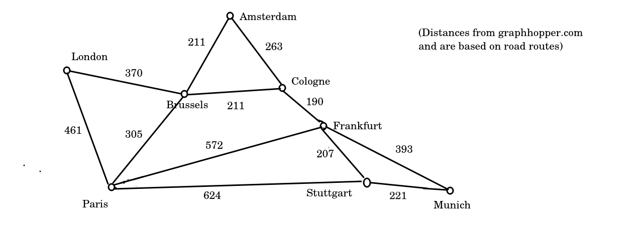
You'll note that the graph is not supposed to be an accurate map, but a representation of key points (nodes; cities here) and the connections between them (edges). You can see a potential routing problem here. How would we route from London to Munich? We could either go via Brussels, Cologne and Frankfurt (3 intermediate stops), or via Paris and Stuttgart (2 intermediate stops) - plus potentially other, longer routes - but which would be the faster or the shorter?

Note how the edges are annotated with the distance (in km) between each node, but we need an efficient way of considering all possibilities and finding the shortest route. Algorithms include:

• Dijkstra's algorithm
• A*

Breadth-first search?

If you think about it we could use a simple breadth-first search to find the shortest path. We could start from a particular node, add all the neighbour nodes to a queue of nodes to be processed, then add their neighbour nodes (ignoring nodes which have already been added), and so on. We would eventually find a route to the node we are looking for.

However this would not necessarily be the shortest route. It would be the route with the least number of intermediate nodes, but this might not be the shortest by distance. We need to consider an algorithm which will take into account the distance between the nodes.

For the assessment, you should not use simple breadth-first search and should find a shortest route by distance.

Dijkstra's algorithm

Dijkstra's algorithm is one of the simplest route-finding algorithms. It can be seen as a modification of breadth-first search which takes into account the distance between nodes. It starts at a given node and then adds all the surrounding nodes to a queue, as for ordinary breadth-first search. Each node is then given a distance from the origin. The distance is the distance of the parent (previous) node plus the distance of the edge leading to the node.

With Dijkstra's algorithm we start at the starting node and gradually explore adjacent nodes. With each node, we pick its neighbour nodes and add them to a data structure known as the open list. The open list is the set of nodes still to be considered. We work through the open list in distance order, so when selecting the next node to consider, we pick the one with the shortest distance from the origin. As soon as we have considered a node from the open list, we remove it, so it's not considered again.

In order to be able to process the nodes in distance order, the open list is typically implemented as a specialised data structure known as a priority queue. A priority queue is an enhanced version of a regular queue; it's a queue which can have a custom ordering, typically a numerical ordering. So in Dijkstra's algorithm we could order the nodes by distance from the starting node.

This is best illustrated by working through an example. Imagine we want to calculate the shortest route from London to Munich, using the graph shown above. We would follow steps shown on the diagram below.

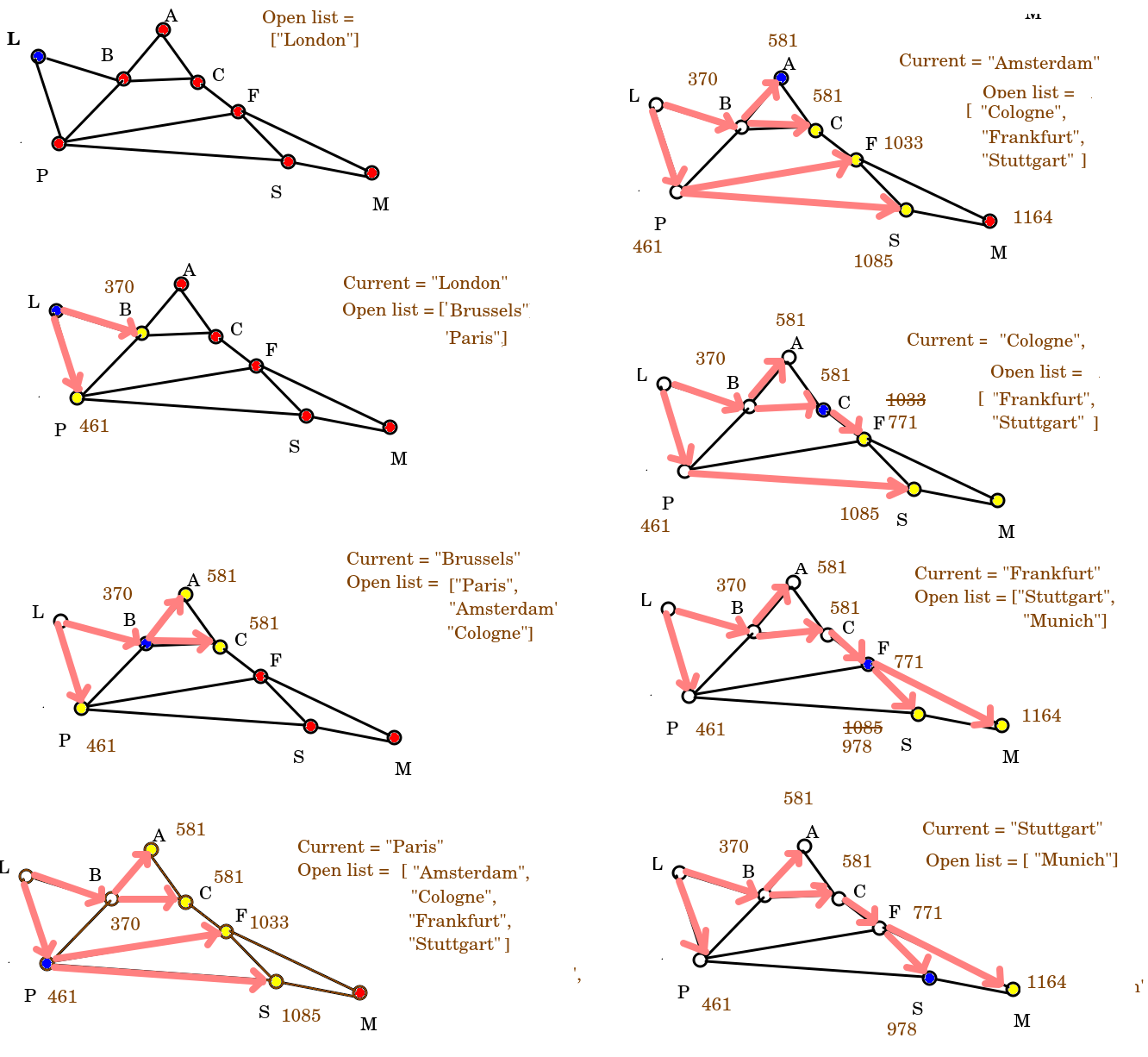
To explain in words, we'd start at the London node and add London's neighbours - Brussels and Paris - to the open list, in distance order (so Brussels first and then Paris, as Brussels is nearer).

When we add a neighbour node, we store its total distance from the origin within the node. So the node for Brussels stores the value 370 km and the node for Paris, 461 km.

Having considered a node, it is then removed from the open list (so as soon as we add the neighbours of London to the open list, we remove London from it).

So we then move on to Brussels as it's the closest-to-London member of the open list (370km), and add its neighbours - Amsterdam and Cologne, which as it happens are exactly the same distance from Brussels. Note that Brussels also has Paris as a neighbour. However, because the distance of London to Paris via Brussels is longer than directly, we do nothing. At this point we remove Brussels from the open list.

Next we consider Paris (461km from London). Paris has Brussels as a neighbour, but Brussels has now been removed from the open list so we ignore it. So we add the two other neighbours of Paris: Frankfurt and Stuttgart, in that order (as Frankfurt is nearer Paris than Stuttgart is) and remove Paris from the open list.

We could then choose from either Amsterdam or Cologne, as both are 581km from London. Let's say we arbitrarily pick Amsterdam, perhaps because it's first in the alphabet. Nothing changes at this step as Brussels is not on the open list, and the route to Cologne via Amsterdam is longer than the direct route. So Amsterdam is removed.

We move onto Cologne. This is where it gets a bit interesting. Two of Cologne's neighbours - Amsterdam and Brussels - have already been considered and removed from the open list. The other, Frankfurt, has a distance (1033km) found from an earlier routing via Paris. However, the distance from London to Frankfurt via Brussels and Cologne is substantially shorter - 771km - so the old Frankfurt distance is replaced by the new. So hopefully you can see that even though there are more intermediate nodes via Brussels and Cologne, the actual distance is shorter. Having done this, we remove Cologne from the open list.

Next is Frankfurt (771km from London). Again some neighbours (Paris and Cologne) have been considered already. However, another - our destination, Munich - is not yet on the open list so we add it. The final neighbour - Stuttgart - is on the open list, but once again, we update its distance from London as the route via Brussels, Cologne and Frankfurt is shorter (978km) than via Paris (1085km). We then remove Frankfurt from the open list.

Then we consider Stuttgart (978km). The only neigbbour still on the open list is Munich, but neither route via Stuttgart is shorter than the route we have already calculated the distance of via Brussels, Cologne and Frankfurt, so we do not alter its distance.

Finally, we are at Munich, and have worked out the shortest route - i.e. the route via Brussels, Cologne and Frankfurt, at 1164km.

If there were more nodes in the graph, we would need to explore them too - just in case we find a shorter route.

How, though, do we get an actual route? We have to now start at the destination (i.e Munich) and work backwards to London, adding each node in turn to the front of a data structure. A deque (double-ended queue) is good for this, as you can add to both the front and the back of a deque. So starting at Munich, the contents of the deque will be, at each step:

To allow this "walking backwards" along the route to occur, each node will need a parent attribute representing its parent node in a Dijkstra routing. So, for example, the parent of Munich will be Frankfurt. The parent of Frankfurt will be Cologne. The parent of Cologne will be Brussels, and the parent of Brussels will be London.

We set the parent attribute when adding nodes to the open list. Each node that we add to the open list has the parent set to the current node, so that, for example, when we add Brussels and Paris to the open list, we set their parent to be the current node, which will be London. Furthermore, when we update a node's distance because we have found a shorter route (e.g. updating Frankfurt's distance due to finding a shorter route via Brussels and Cologne than via Paris) we also change the parent, so that in this example, the parent of Frankfurt will be changed from Paris to Cologne.

Pre-calculation of all paths

This simple illustration of Dijkstra simply calculated the path from one origin to one destination. However, Dijkstra is generally used to pre-calculate the path from an origin node to every other node, and store each path for later use. This improves the efficiency, as if you want to calculate the route multiple times from a given origin node to another node, you can use the pre-calculated route rather than having to recalculate it each time.

Implementing a priority queue in Python

You can easily implenent a priority queue in Python using functions from the heapq module. Priority queues are implemented using a specific type of sorted tree known as a heap, hence the name. A heap is a tree "for which every parent node has a value less than or equal to any of its children" (see the Python docs). Here is a simple example of creating a priority queue and then removing items from it. Note how we use heappush() to add to the queue and heappop() to remove from the front of it. See the documentation here

Coding Dijkstra

Using the notes to help you, implement an initial attempt at Dijkstra's algorithm to find the shortest route from London to Munich. You will need to create Node and Edge classes to represent nodes and edges respectively, and a `Graph' class to represent the graph.

Once this is done, test it out by allowing the user to enter a city, and then display the path from London to the user's chosen city.

Some hints:

• your Node class should contain dist (containing the distance from the start), together with a name, a parent (set to None), and an edges list. The distance should initally be a large number such as sys.maxsize (for which you need to import sys) so that when updated, the new value will always be less than the old.

• your Node class should also contain an in_open_list boolean, to indicate whether the node is currently in the open list. It should be false initially, but set to true when added to the open list. This is to prevent duplicates of the same node being added to the open list.
• Node should also have an removed boolean, set to False originally. This will be set to True when the node is removed from the front of the open list, to indicate it does not need to be considered again.
• your Edge class should contain start (the start node), end (the end node) and dist (the edge distance) and an appropriate initialiser method to initialise these three attributes.
• your Graph class should also contain an add_edge() method. This should take as parameters start, end and dist, representing the start node, end node and distance. It should then call the add_edge() method of Node twice:
  • first create an Edge going from the start to end and add it to the start node's edges.
  • then create an Edge going from the end to start and add it to the end node's edges. This way you have a two-way connection between nodes which will be more efficient,
• your Graph should also have a dijkstra() method. This should take the start and end nodes as parameters and implement the algorithm.

Answer to exercise 1

• The while loop must continue until the open list (priority queue) is empty which means we cannot find a valid route, or (in this first attempt) until we reach the destination. (This will be changed later, though).

• We need to remove the first node from the priority queue and set that as the current node.

• The inner loop must loop through all the edges of the current node, and consider the end node of each edge. Potentially each end node will be added to the priority queue - we will use the next exercise to explore this.

Answer to exercise 2

• We must check that the neighbour node hasn't already been removed from the open list via the removed attribute. If it has, we don't even need to consider it.

• The weight (distance) of each neighbour node needs to be set equal to the distance of the current node plus the weight of the edge.

• If the new distance is greater than the existing distance, we should not update it as we have not found a shorter route.

• We must set its parent to the current node, so that we can trace back the route later. Also, we must add the neighbour to the open list if it's not there already, and set in_open_list to True.

• We must start at the end node, backtrack to the start, and using a deque (see below) add each successive parent to the front of the deque to get a route.

Having obtained a route, we can then store it in a dictionary within the graph for later use.

Using a deque to backtrack from end to start, and obtain a route

Use a deque to loop back from the end node to start once you've found the route, e.g:

If the end node has no parent, what can you conclude?

You will get a problem with the priority queue because, when comparing values, the queue will not know how to compare Nodes. You can compare nodes by distance by overloading the < operator for Nodes. Here is how to do this. Add a __lt__() magic method to your Node class which compares Nodes by name:

Using the graph of European cities above, test it out and see if it works on London to Munich.

Further Exercise - Improving our first attempt at Dijkstra

Can you think of a more efficient way to perform Dijkstra if you want to find the routes from London to every other city, so this can be cached for later use?

We could repeat the route finding we used for Munich to each city, but this would be inefficient. We can improve upon this. How?

Answer

If you think about it, when you perform Dijkstra's algorithm to route from London to Munich, you also find the shortest path to every intermediate city. So it would be wasteful and inefficient to then recalculate the shortest path to the other cities.

What we can do instead is to modify our Dijkstra method to always keep looping until the open list is empty. By doing this, we ensure that we find routes to every other node.

To achieve this, we simply remove the destination parameter from our Dijkstra method and modify our loop to remove the condition checking whether the current node is equal to the destination. This will cause our Dijkstra method to find routes to all other nodes. We then only run the method once per origin.

However, the code which back-tracks from destination to origin using a deque still needs to be run for each of the other nodes, so we can find a forward path from the origin to each node. So it needs to be separated out into its own method. We run this for each of the other nodes and then cache each route in, for example, a dictionary indexed by destination name within the Graph class.

Modify your Dijkstra algorithm to do this.